RLVR Reward Landscape
zooming into the local reward landscape around a policy
tl,dr
- We study 2-dimensional slices of the parameter space around GRPO checkpoints and compare the local surrogate loss, reward, and KL divergence induced by perturbations of the current policy.
- We find that high-reward policies occupy a small region of the local slice and are strongly concentrated near the current policy in distribution space, as measured by the KL divergence.
This work is a WIP case study. The goal is to probe one concrete setup and surface hypotheses about local reward geometry that could be tested across more models, tasks, perturbation scales, and seeds.
Introduction
Reinforcement Learning with Verifiable Rewards (RLVR) is often motivated as a way to improve pretrained large language models (LLMs) on specific tasks through trial-and-error
A growing debate asks whether RLVR finds and elicits new reasoning capabilities from the models or whether it simply reallocates probability mass towards correct reasoning trajectories that were already accessible to the base models
Most existing analyses study the exploration-exploitation question through output-based evaluations, which reveal what a policy can sample but not how training reshapes the nearby policy landscape. In alignment with this trust region view and inspired by loss landscape visualization methods
Methodology
Overview
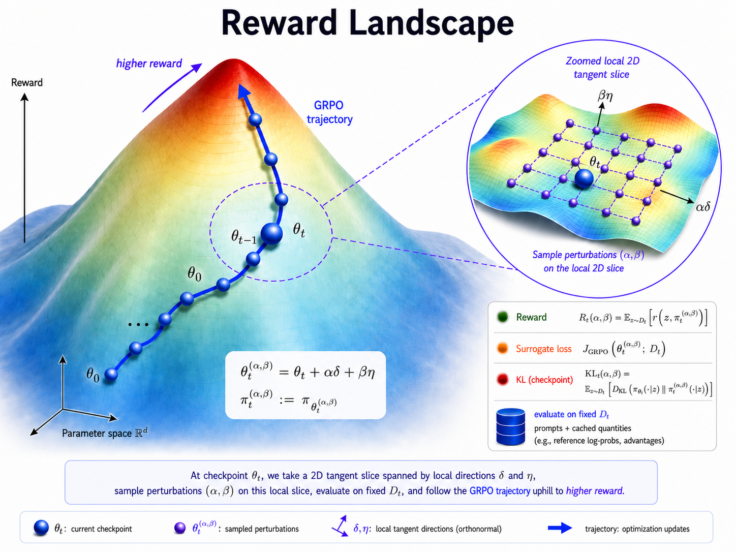
The experiment has two stages. First, we train Qwen2.5-0.5B-Instruct with GRPO on Alphabet-sort, saving intermediate checkpoints throughout training. Second, we freeze each checkpoint and probe a local two-dimensional slice of the surrounding parameter space. Each point in this slice defines a counterfactual nearby policy, which we evaluate by surrogate loss, reward, and KL divergence from the original checkpoint policy.
In this experiment, GRPO refers to the clipped token-level policy-gradient surrogate used during training. For a batch $\mathcal{B}$, let $y_{i}$ be ith sampled completion in the group and let $\hat{A}_{i}$ be the group-relative advantage. With
\[\rho_{i,t}(\theta) = \frac{\pi_{\text{train}}(y_{i, t} | x, y_{i < t}; \theta)}{\pi_{\text{infer}}(y_{i, t} | x, y_{i < t}; \theta_{old})}\]the GRPO objective used here is
\[J_{\mathrm{GRPO}}(\theta) = \sum_{x\sim \mathbb{D}, {y_i}_{i=1}^N \sim \pi_{infer}} \min\!\left[ \frac{1}{\sum_{i=1}^N |y_i|} \sum_{i=1}^N \sum_{t=1}^{|y_i|} (\rho_{i}(\theta)\hat{A}_{i}, \operatorname{clip}\!\left(\rho_{i}(\theta), 1-\epsilon, 1+\epsilon\right)\hat{A}_{i}) \right].\]Training checkpoints
Let $\theta_t$ denote the model parameters during training at step $t$, and let $\pi_{\theta_t}$ denote the corresponding policy. Using GRPO, we update the policy on the Alphabet-sort training environment, where each prompt asks the model to sort an increasing list of names across multiple turns. At a high level, the update takes the form
\[g_t = \nabla_{\theta} J_{\mathrm{GRPO}}(\theta_t), \qquad \theta_{t+1} = \theta_t + \omega_t g_t,\]where $\omega_t$ is the step size.
We train for 150 steps and save checkpoints every 10 steps and these checkpoints are then treated as fixed objects during landscape construction.
Evaluation set construction
For landscape evaluation, we use a fixed prompt set
\[\mathcal{D} = \{x_i\}_{i=1}^{N},\]where $N = 1024$. The prompts are sampled from the Alphabet-sort environment. We use the same $\mathcal{D}$ for every checkpoint so that changes in the measured landscapes reflect changes in the policy neighborhood around $\theta_t$, not changes in the evaluation prompts.
Landscape construction
To study the local geometry around checkpoint $\theta_t$, we sample two random direction tensors $\delta_t$ and $\eta_t$. Each direction is normalized per weight tensor relative to the corresponding tensor norm in $\theta_t$. For sweep coefficients $(\alpha, \beta)$ on a two-dimensional grid, we define the perturbed parameters
\[\theta_t^{(\alpha, \beta)} = \theta_t + \alpha \delta_t + \beta \eta_t,\]and the associated perturbed policy
\[\pi_t^{(\alpha, \beta)} := \pi_{\theta_t^{(\alpha, \beta)}}.\]We evaluate $\pi_t^{(\alpha, \beta)}$ on a $21 \times 21$ grid with $\alpha, \beta \in [-0.05, 0.05]$, giving 441 perturbed policies per checkpoint. For each checkpoint, the sampled directions are fixed across the full grid, and perturbations are applied to all trainable weights. This defines a local two-dimensional parameter-space slice around $\theta_t$.
Landscape metrics
For each checkpoint $t$ and each grid point $(\alpha, \beta)$, we evaluate three quantities:
-
GRPO surrogate objective $J_{\mathrm{GRPO}}(\theta_t^{(\alpha,\beta)})$, evaluated on completions sampled from the unperturbed checkpoint policy $\pi_{\theta_t}$ using prompts from the fixed set $\mathcal{D}$;
-
mean rollout reward
\[R_t(\alpha, \beta) = \mathbb{E}_{x \sim \mathcal{D}} \left[ r\!\left(x, \pi_t^{(\alpha, \beta)}\right) \right],\]where $r(x, \pi)$ is the verifier-based reward obtained by rolling out policy $\pi$ on prompt $x$;
-
KL divergence from the checkpoint policy
\[\mathrm{KL}_t(\alpha, \beta) = \mathbb{E}_{x \sim \mathcal{D}} \left[ D_{\mathrm{KL}}\!\left( \pi_{\theta_t}(\cdot \mid x) \,\|\, \pi_t^{(\alpha, \beta)}(\cdot \mid x) \right) \right].\]
Together, these measurements define a local loss, reward, and divergence landscape around checkpoint $\theta_t$. Repeating this procedure across training checkpoints lets us track how the local high-reward region evolves over the course of RLVR training.
Takeaways
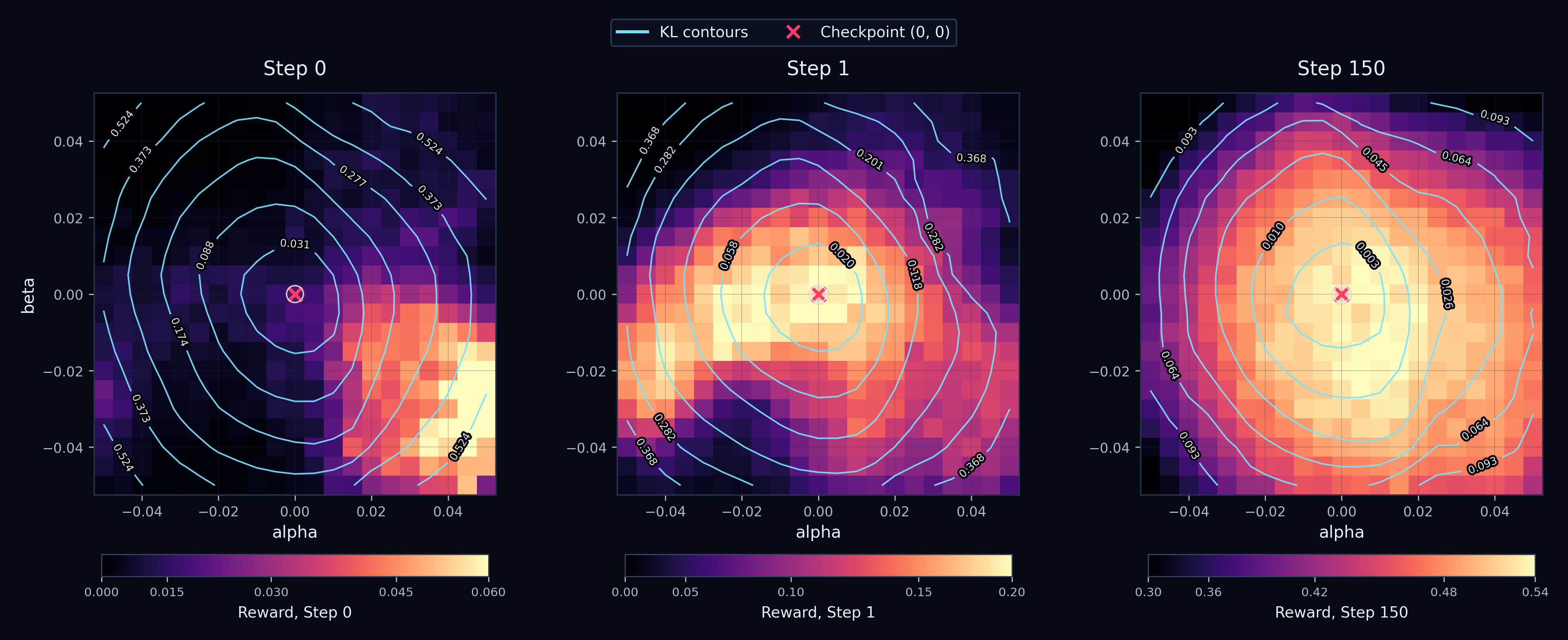
T1: High-reward policies become concentrated near the current policy.
At each checkpoint $t$, we measure the KL divergence between the current policy and pertubed policy $\theta_t^{(\alpha, \beta)}$, all 441 of them, as well as the reward on $D$. A useful but relatively trivial baseline is that low-KL policies are always concentrated near the current checkpoint - the KL is measured relative to the current policy, so it makes sense that perturbations that leave the policy distribution almost unchanged naturally sit close to $\pi_{\theta_t}$ in distribution space.
The nontrivial observation is that reward becomes concentrated around the current checkpoint too! High-reward perturbed policies are not spread uniformly across the local slice. Instead, they tend to appear in the same region where the perturbed policy remains close to the checkpoint distribution.
In Figure 1, reward heatmaps and KL contours are plotted over the local parameter slice. If KL localization were the only effect, we would expect the KL contours to be centered near the checkpoint, but reward could still peak elsewhere. Instead, we observe that the high-reward region increasingly overlaps with the low-KL region.
We further quantify this alignment between reward and KL by measuring the Pearson correlation between both terms across the perturbation grid. A negative KL–reward correlation means that, among locally reachable policies, the policies farther from the checkpoint distribution tend to receive lower reward, while policies closer to the checkpoint tend to receive higher reward.
Figure 2 makes this point across checkpoints. The KL–reward correlation becomes negative early in training, by step 10, indicating that within the reachable neighborhood, moving farther away from the current policy tends to hurt reward.
The above observation is interesting as it opens up the question of whether exploration is meant to produce trajectories that are far or close in distribution space. We explore this further in T3.
Which policy the optimizer chooses is another question.
T2: The concentration happens early in the training.
One possible explanation for T1 is that the concentration is just a late-training effect: once the model has already improved, most high-reward perturbations would naturally be small deviations from the current policy. Under this view, the negative KL-reward correlation would mainly appear after the reward landscape has already settled around a strong checkpoint.
This makes the timing important. If localization only appears near the end of training, it would look more like a consequence of convergence. If it appears in the first few updates, then RLVR may be moving the model into a locally favorable region of policy space much earlier than the final reward curve would suggest, analogous to entering a low-loss basin in supervised learning.
To investigate this, we zoom in on the first 10 training steps. Figure 3 shows that the KL-reward correlation becomes strongly negative almost immediately, suggesting that the local high-reward region becomes concentrated near the checkpoint policy early in training.
T3: RLVR increasingly behaves like local exploitation around the current policy rather than broad exploration.
A natural reading of T1 and T2 is that RLVR quickly becomes local. High-reward perturbations are not spread broadly across the sampled neighborhood, they are concentrated near the checkpoint policy in KL terms.
How does exploration fit into this? A reasonable conclusion is that the notion of broad exploration over the entire policy space isn’t supported by GRPO and by extension, it’s derivative algorithms. They seem to rather exploit the local reachable low KL neighbourhood around the current policy.
The evidence seems to suggest that after a small number of updates, useful exploration may be constrained to a low-KL neighborhood of the current policy. In that sense, RLVR may behave less like broad exploration over policy space and more like exploitation within a locally reachable region.
Limitations
-
2D slices are lossy views of a high-dimensional object. The landscape is a 2-dimensional slice though a ~490M-dimensional space. This is useful for probing local structure, but it is still an approximation as the slice may miss directions where reward, loss, or KL behave differently.
-
The perturbation scale matters. The coefficients $\alpha$ and $\beta$ control how far we zoom out from the checkpoint. In early experiments, larger ranges such as $\pm 0.1$ pushed most perturbed policies into regions with zero reward. Much smaller ranges kept policies too close to the checkpoint, producing too little variation in reward and KL. The range $[-0.05, 0.05]$ gave the most useful resolution for this setup, but this scale is a methodological choice that could be tuned further.
-
The model and task scope are limited. All results here use Qwen2.5-0.5B-Instruct on Alphabet-sort. The task was chosen because it is simple enough for this model and reaches useful reward levels with relatively few training tokens, making the landscape evaluation computationally feasible. Its partial-credit reward also matters: although rewards lie between 0 and 1, they are not strictly binary, so the landscape still contains useful variation.
The above factors interact. In early GSM8K experiments with binary rewards on Qwen2.5-0.5B, the same $\pm 0.05$ perturbation range was too zoomed out: most perturbed policies received zero reward. This suggests that model scale, task difficulty, reward granularity, and perturbation scale may all affect the observed local geometry and exploration-exploitation behavior under RLVR.
Appendix
Configuration summary
Training configuration
| Component | Value |
|---|---|
| Base model | Qwen/Qwen2.5-0.5B-Instruct |
| Training environment | Alphabet-sort with min_turns = 2, max_turns = 2 |
| RL algorithm | GRPO |
| Optimizer | AdamW |
| Learning rate | 6e-6 |
| Batch size | 512 |
| Rollouts per example | 16 |
| Sequence length | 4096 |
| Sampling max tokens | 128 |
| Mask truncated completions | false |
| Advantage type | grpo |
| Advantage epsilon | 1e-8 |
| Loss type | grpo |
| Clip epsilon | 0.2 |
| KL coefficient | 0.0 |
| Training steps | 150 |
| Eval interval | Every 10 steps |
| Eval examples | 128 |
| Eval rollouts per example | 1 |
| Eval environment | Alphabet-sort with min_turns = 2, max_turns = 2, seed = 2001 |
| Eval sampling | max_tokens = 128, temperature = 0.7 |
| Extra logging interval | Every 30 steps |
Landscape configuration
| Component | Value |
|---|---|
| Evaluation environment | Alphabet-sort |
| Environment args | min_turns = 2, max_turns = 2, seed = 12345 |
| Buffer seed | 12345 |
| Batch size | 1024 |
| Rollouts per example | 16 |
| Sampling max tokens | 512 |
| GRPO clip epsilon | 0.2 |
| Grid range | $\alpha, \beta \in [-0.05, 0.05]$ |
| Grid resolution | $21 \times 21$ |
| Metrics | GRPO surrogate loss, rollout reward, KL divergence |
Acknowledgment
I am super grateful to Andreas Chollet (for sponsoring compute on this), Daniel David and Professor Ivanov for feedback and insightful questions on earlier drafts of this work.
Prime-Intellect for their easy to use RL library and Qwen team for banger models.